

How to Create ARIMA Model Forecasting BTCUSD in Python Part 2
This post is a continuation of part 1. Since most of the prerequisites have been mentioned in part 1, I would recommend you to glimpse through and come back later.
The Box-Cox transformation is a family of power transformations indexed by a parameter lambda. By definition, when lambda is zero, box-cox is actually using natural log to do the transformation. Since taking natural log is basically a special case for Box-Cox transformation, we are going to examine the difference on our data. Before we start, let us create a function which can help us to understand the results later.
def run_box_cox(pd_dataframe):
    """
    Perform Box-Cox Transformation on column 'price'
    Save the resutls into a new column 'price_box'
    Save lmbda into a new column 'lmbda'
    """

    if 'Day' in str(pd_dataframe.index.freq):
        frequency = 'Daily'
    elif 'Week: weekday=6' in str(pd_dataframe.index.freq):
        frequency = 'Weekly'
    elif '2 * Weeks: weekday=6' in str(pd_dataframe.index.freq):
        frequency = 'Bi-weekly'
    elif 'MonthEnd' in str(pd_dataframe.index.freq):
        frequency = 'Monthly'

    sns.set(style="darkgrid")
    f, axes = plt.subplots(2, 2, figsize=(12, 10), sharex=False)

    ax1 = axes[0, 0]
    prob = stats.probplot(pd_dataframe['price'], dist=stats.norm, plot=ax1, fit=False)
    ax1.set_title('Probability Plot Before Transformation')

    ax2 = axes[0, 1]
    # Perform Box-Cox Transformation
    box_cox, lmbda = stats.boxcox(pd_dataframe['price'])
    # Record new column 'price_box' in pd
    pd_dataframe['price_box'] = pd.Series(box_cox, index=pd_dataframe.index)
    # Record lmbda in pd
    pd_dataframe['lmbda'] = lmbda
    prob = stats.probplot(box_cox, dist=stats.norm, plot=ax2, fit=False)
    ax2.set_title('Probability Plot After Transformation')

    ax3 = axes[1, 0]
    sns.kdeplot(pd_dataframe['price'], shade=True, ax=ax3, label='KDE Price')
    ax3.set_title('KDE Plot Before Transformation')

    ax4 = axes[1, 1]
    sns.kdeplot(box_cox, shade=True, ax=ax4, label='KDE Price Box', color='r')
    ax4.set_title('KDE Plot After Transformation')

    f.suptitle('BTCUSD {} Price Box-Cox Transformation'.format(frequency), fontsize=16)
    f.subplots_adjust(top=0.91, hspace=0.3)

    plt.show()
While we are at it, let us also create an inverse function for Box-Cox transformation.
def inverse_box_cox(time_series, lmbda):
    """
    Inverse Box-Cox Transformation
    """
    if lmbda == 0:
      return(np.exp(time_series))
    else:
      return(np.exp(np.log(lmbda*time_series+1)/lmbda))
Run it through our data sets and see what happens.
for df in df_list:
    run_box_cox(df)
A probability plot (a sample vs a theoretical distribution) is not a QQ-plot. A QQ-plot compares two samples. Although many resources are contradicting with NIST definition, plotting a sample is essentially the same as using the empirical distribution function.
Nevertheless, we are plotting one dsitribution's quantiles against another.
A more thorough discussion can be found on stackoverflow.
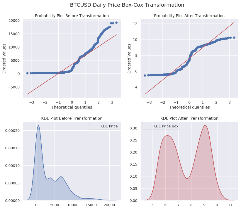

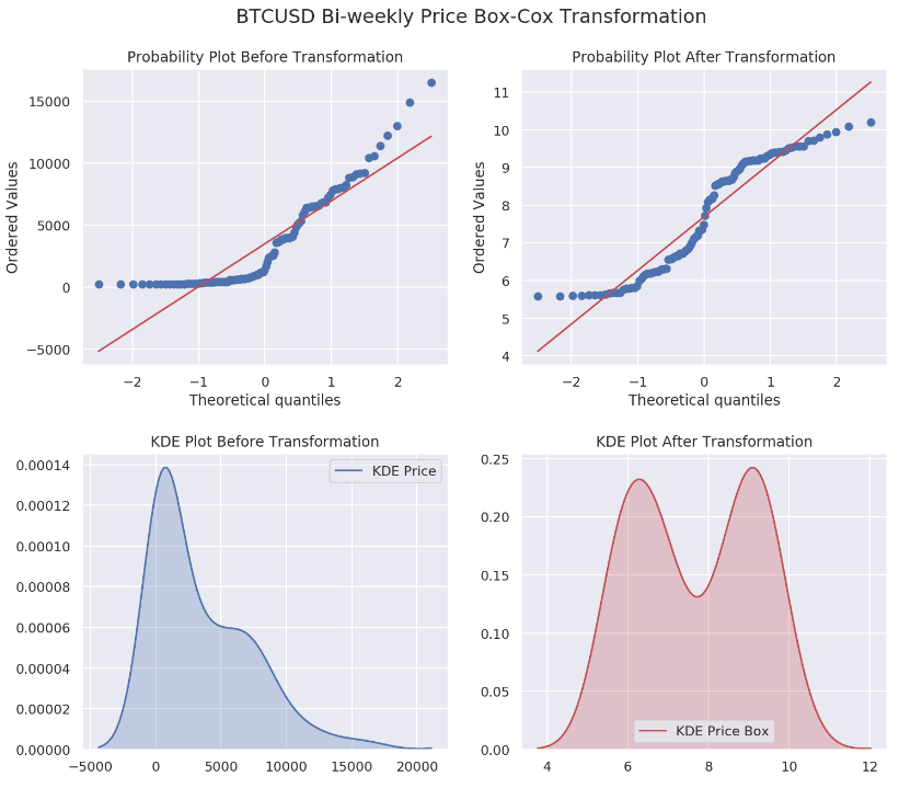
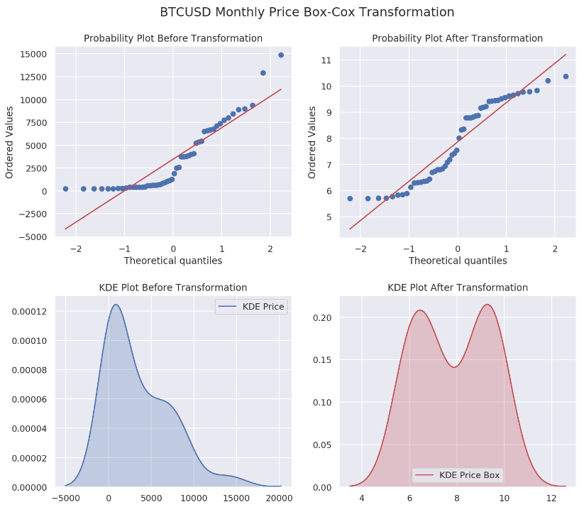
From the results above, we have four different lmbda values of 0.00766, 0.0102, 0.0101 and 0.0158 for daily, weekly, bi-weekly and monthly data sets, respectively. Not that quite close to zero, aren’t they?
After applying Box-Cox with a particular value of lambda, the process may look stationary. However, it is often to see the series does not appear to be stationary even if after applying the Box-Cox transformation.
Unfortunately, our data is still far away from be stationary after Box-Cox transformation. The next step is differencing. For the sake of this series, we are not going to dive into seasonality. Instead, we will apply the first-order differencing. I am sure it will be quite fascinating to investigate the seasonality of our data, but that will be left for another future post.
# Take the first-order difference for our data sets
print('Box-Cox Transformed Price First-order Differencing ADF Test')
for df in df_list:
    if 'Day' in str(df.index.freq):
        frequency = 'Daily'
    elif 'Week: weekday=6' in str(df.index.freq):
        frequency = 'Weekly'
    elif '2 * Weeks: weekday=6' in str(df.index.freq):
        frequency = 'Bi-weekly'
    elif 'MonthEnd' in str(df.index.freq):
        frequency = 'Monthly'
    df['price_box_diff_1'] = df['price_box'] - df['price_box'].shift(1)
    print('{} : p={}'.format(frequency, adfuller(df.price_box_diff_1[1:])[1]))
Box-Cox Transformed Price First-order Differencing ADF Test
Daily : p=1.4350549191553701e-27
Weekly : p=1.9953078780986301e-19
Bi-weekly : p=1.4329230115109643e-09
Monthly : p=3.834668265736053e-05
Looks good! Now it is time to investigate autocorrelations (ADF) and partial autocorrelations (PADF). Honestly, I have been struggling to understand those two. Thanks to ritvikmath’s video, I have a much clearer picture of what I am getting myself into. Anyways, let us create a function called run_acf_pacf.
def run_acf_pacf(time_series, title, lags=40):

    sns.set(style='darkgrid')
    fig_acf_pacf = plt.figure(figsize=(21,7))

    # Start time series from the first valid entry
    first_valid_date = time_series.first_valid_index()
    time_series = time_series.loc[first_valid_date:]

    # ACF Chart
    ax_acf = plt.subplot2grid((5, 10), (0, 0), rowspan=3, colspan=5)
    plot_acf(time_series, lags=lags, ax=ax_acf, lw=1)
    plt.title('', fontsize=12)
    plt.yticks(fontsize=10)
    plt.xticks(fontsize=10, rotation=0)
    plt.title('Estimated Autocorreclations (ACF)', fontsize=14)

    # PACF Chart
    ax_pacf = plt.subplot2grid((5, 10), (0, 5), rowspan=3, colspan=5)
    plot_pacf(time_series, lags=lags, ax=ax_pacf, lw=1)
    plt.title('', fontsize=12)
    plt.yticks(fontsize=10)
    plt.xticks(fontsize=10, rotation=0)
    plt.title('Estimated Partial Autocorreclations (PACF)', fontsize=14)

    plt.subplots_adjust(left=0.1, bottom=0.15, right=1, top=0.90, wspace=0.7, hspace=0)
    plt.suptitle(title, fontsize=20)
    plt.show()
Similarly, we run ACF and PACF through those four data sets.
for df in df_list:
    run_acf_pacf(df['price_box_diff_1'], lags=40)
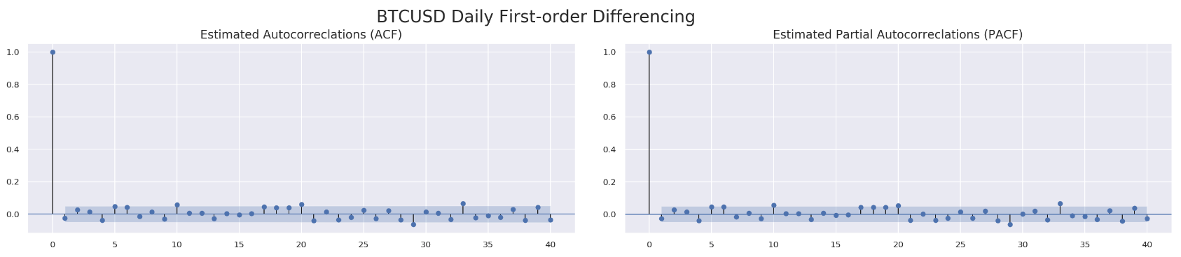
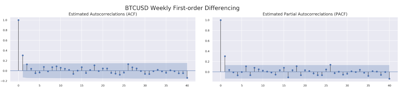
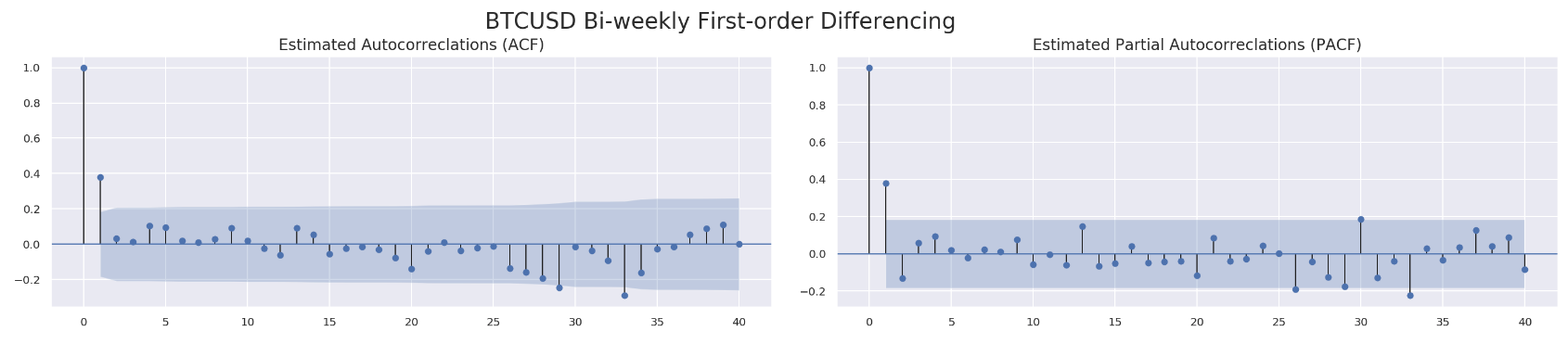
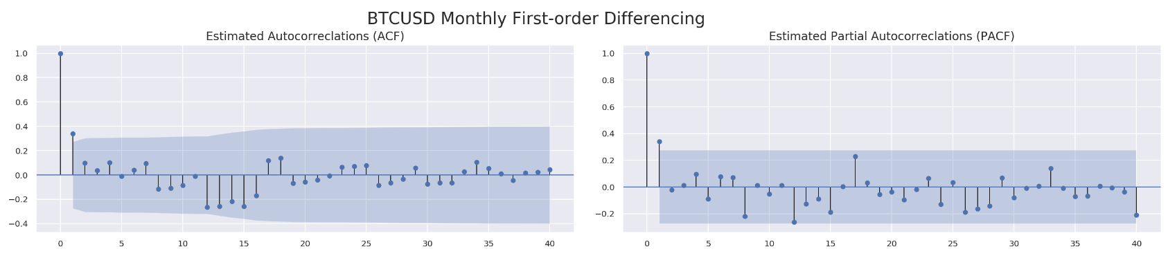
So far we know we are going to stick with d=1. What about p and q? For q, all four data sets seem to have a value less than 3 based on estimated autocorrelations. As to p, we might be able to get away with a value less than 10 according to PACF results. We are going to utilize model selectors to pick the best one from a range of (p, d, q) combinations. Here is how each model selector works. The selector measures how well a model fits the data while taking into account the overall complexity of the model. A model that fits the data very well while using lots of features will be assigned a larger score than a model that uses fewer features to achieve the same goodness-of-fit. Therefore, we are interested in finding the model that yields the lowest value. The model selectors include Akaike Information Criterion (AIC), Bayesian Information Criterion (BIC) and Hannan–Quinn Information Criterion (HQIC). Normally, those three selectors will agree with each other. In case they do not, our function will just pick the one with at least two confirmations.
Here is the code for selecting best parameters.
def select_best_params(pd_dataframe):
    """
    Return best params (p, d, q) for the data sets with different frequences
    Evaluate the scores from AIC, BIC and HQIC
    Select the most favorable one among those three model selection criteria
    """
    if 'Day' in str(df.index.freq):
        frequency = 'Daily'
    elif 'Week: weekday=6' in str(df.index.freq):
        frequency = 'Weekly'
    elif '2 * Weeks: weekday=6' in str(df.index.freq):
        frequency = 'Bi-weekly'
    elif 'MonthEnd' in str(df.index.freq):
        frequency = 'Monthly'
    print('BTCUSD {} 1st Order Differencing Best (p, d, q):'.format(frequency))

    # Initial approximation of parameters
    ps = range(0, 10)
    ds= range(1, 2)
    qs = range(0, 3)
    parameters = product(ps, ds, qs)
    parameters_list = list(parameters)

    # Model Selection
    best_params = []
    aic_results = []
    bic_results = []
    hqic_results = []
    best_aic = float("inf")
    best_bic = float("inf")
    best_hqic = float("inf")
    warnings.filterwarnings('ignore')
    for param in parameters_list:
        try:
            model = SARIMAX(pd_dataframe['price_box'], order=(param[0], param[1], param[2])).fit(disp=-1)
        except ValueError:
            continue

        aic_results.append([param, model.aic])
        bic_results.append([param, model.bic])
        hqic_results.append([param, model.hqic])

    aic_df = pd.DataFrame(aic_results)
    aic_df.columns = ['params', 'aic']
    best_params.append(aic_df.params[aic_df.aic.idxmin()])
    print('AIC best param: {}'.format(aic_df.params[aic_df.aic.idxmin()]))

    bic_df = pd.DataFrame(bic_results)
    bic_df.columns = ['params', 'bic']
    best_params.append(bic_df.params[bic_df.bic.idxmin()])
    print('BIC best param: {}'.format(bic_df.params[bic_df.bic.idxmin()]))

    hqic_df = pd.DataFrame(hqic_results)
    hqic_df.columns = ['params', 'hqic']
    best_params.append(hqic_df.params[hqic_df.hqic.idxmin()])
    print('HQIC best param: {}'.format(hqic_df.params[hqic_df.hqic.idxmin()]))

    for best_param in best_params:
        if best_params.count(best_param)>=2:
            print('Best Param Selected: {}'.format(best_param))
            return best_param
Again, let us run it through our data sets and see what we can find.
for df in df_list:
    best_param = select_best_params(df)
BTCUSD Daily 1st Order Differencing Best (p, d, q):
AIC best param: (6, 1, 0)
BIC best param: (1, 1, 0)
HQIC best param: (1, 1, 0)
Best Param Selected: (1, 1, 0)
BTCUSD Weekly 1st Order Differencing Best (p, d, q):
AIC best param: (1, 1, 0)
BIC best param: (1, 1, 0)
HQIC best param: (1, 1, 0)
Best Param Selected: (1, 1, 0)
BTCUSD Bi-weekly 1st Order Differencing Best (p, d, q):
AIC best param: (0, 1, 1)
BIC best param: (0, 1, 1)
HQIC best param: (0, 1, 1)
Best Param Selected: (0, 1, 1)
BTCUSD Monthly 1st Order Differencing Best (p, d, q):
AIC best param: (1, 1, 0)
BIC best param: (1, 1, 0)
HQIC best param: (1, 1, 0)
Best Param Selected: (1, 1, 0)
Interestingly, almost all three model selectors render the same param for each data set, except for daily data ((6, 1, 0) vs. (1, 1, 0)). We can test (6, 1, 0) for daily data separately and see if there is anything we could miss.
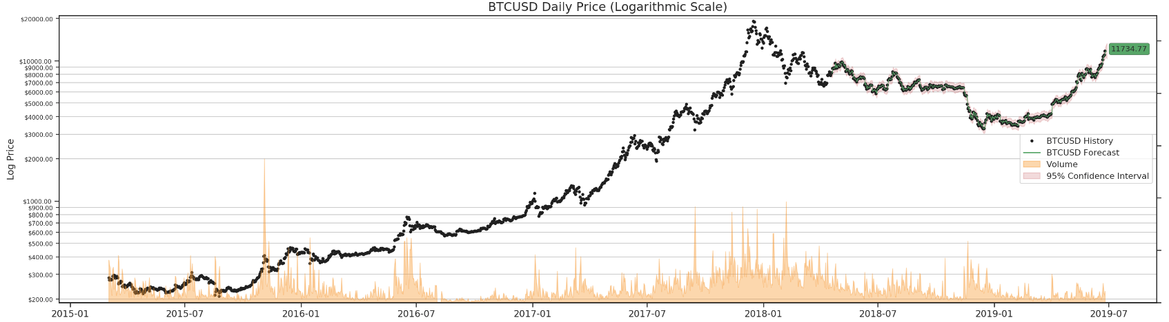
Now, it is time to build the function for rendering results. We are going to break down each data set into two groups: training data and testing data. After training the model, we can use one-step-ahead method to do in-sample and out-of-sample (3 steps) forecasting. You might also heard of dynamic forecasting method. Unfortunately, I could not figure out how it works in my setup. Please DO let me know if you know how. Much appreciated!
Dynamic: prior to this observation, true endogenous values will be used for prediction; starting with this observation and continuing through the end of prediction, forecasted endogenous values will be used instead.
Basically it means you can set up a certain timestamp and ask the model to forecast the next value based on previous forecasted valude if dynamic mode is enabled. Otherwise, the model will use the observed/expected value instead. By definition, the dynamic model might travel well off the charts, but it would be interesting to see how it turns out in our model.
Here is our render function.
def render_results(pd_dataframe, params=None, steps=3):
    """
    In-sample one-step-ahead predictions
    Use 2015~2017 data to train
    Use 2018~2019 data to test

    Out-of-sample predictions
    Forecast 3 steps
    """
    # lmbda
    lmbda=pd_dataframe.lmbda[0]

    # Params
    if not params:
        params = select_best_params(pd_dataframe)

    # Data
    training_ts = pd_dataframe.loc['2015':'2017', 'price_box']
    testing_ts = pd_dataframe.loc['2018':'2019', 'price_box']

    # Train the model
    training_model = SARIMAX(endog=training_ts, order=params)
    training_model_fit = training_model.fit(disp=False)

    # Test the model
    testing_model = SARIMAX(endog=testing_ts, order=params)
    testing_model_fit = testing_model.smooth(training_model_fit.params)

    # Prediction
    prediction_wrapper = testing_model_fit.get_prediction(start=int(testing_model.nobs * 0.2), end=testing_model.nobs + steps, full_reports=True)
    prediction_ci = prediction_wrapper.conf_int()
    prediction = prediction_wrapper.predicted_mean

    # Inverse Box-Cox Transformation
    prediction_inversed = inverse_box_cox(prediction, lmbda)
    prediction_ci_inversed = inverse_box_cox(prediction_ci, lmbda)

    # Add prediction  and confidence interval back to the original dataframe

    if 'Day' in str(pd_dataframe.index.freq):
        frequency = 'Daily'
        future_dates = pd.date_range(pd_dataframe.index[-1] + timedelta(days=1), periods=steps, freq='D')
    elif 'Week: weekday=6' in str(pd_dataframe.index.freq):
        frequency = 'Weekly'
        future_dates = pd.date_range(pd_dataframe.index[-1] + timedelta(weeks=1), periods=steps, freq='W')
    elif '2 * Weeks: weekday=6' in str(pd_dataframe.index.freq):
        frequency = 'Bi-weekly'
        future_dates = pd.date_range(pd_dataframe.index[-1] + timedelta(weeks=2), periods=steps, freq='2W')
    elif 'MonthEnd' in str(pd_dataframe.index.freq):
        frequency = 'Monthly'
        future_dates = pd.date_range(pd_dataframe.index[-1] + timedelta(days=30), periods=steps, freq='1M')

    future = pd.DataFrame(index=future_dates, columns=pd_dataframe.columns)

    pd_dataframe = pd.concat([pd_dataframe, future])
    pd_dataframe['forecast price_box'] = prediction
    pd_dataframe['lower price_box'] = prediction_ci.iloc[:, 0]
    pd_dataframe['upper price_box'] = prediction_ci.iloc[:, 1]
    pd_dataframe['forecast'] = prediction_inversed.round(2)
    pd_dataframe['lower forecast'] = inverse_box_cox(pd_dataframe['lower price_box'], lmbda)
    pd_dataframe['upper forecast'] = inverse_box_cox(pd_dataframe['upper price_box'], lmbda)

    # Plot
    make_log_price_chart(pd_dataframe, frequency=frequency)
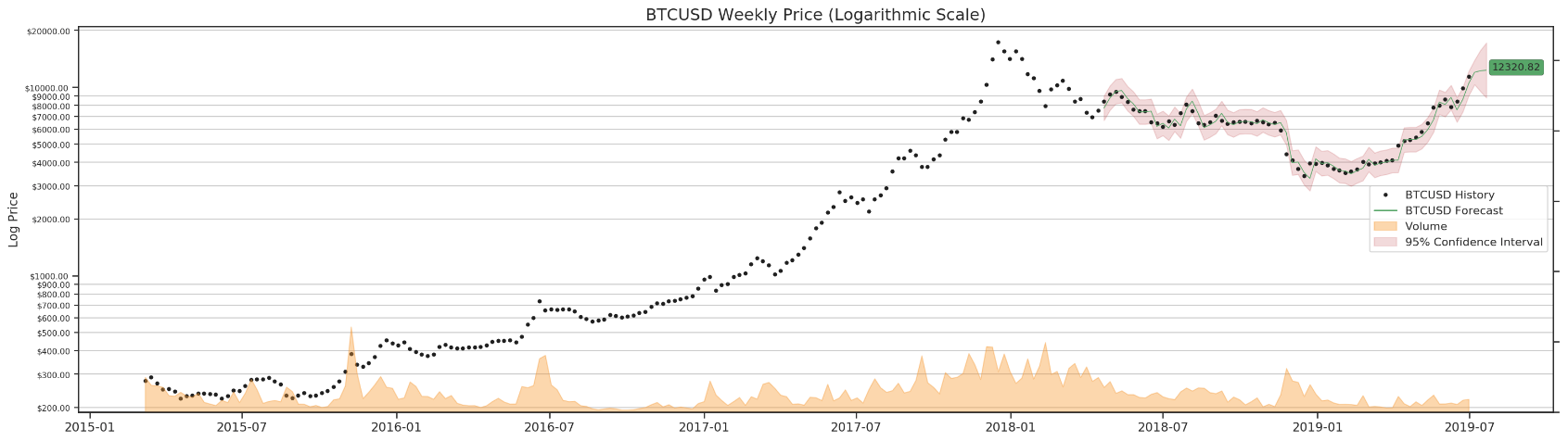
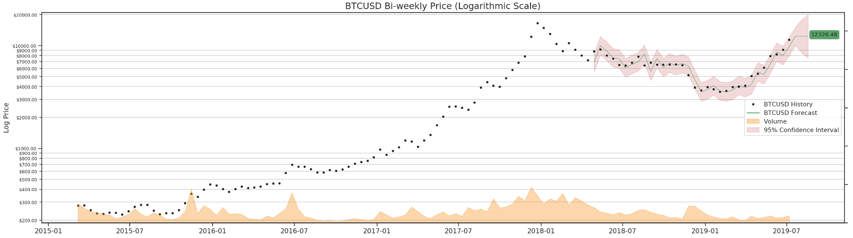
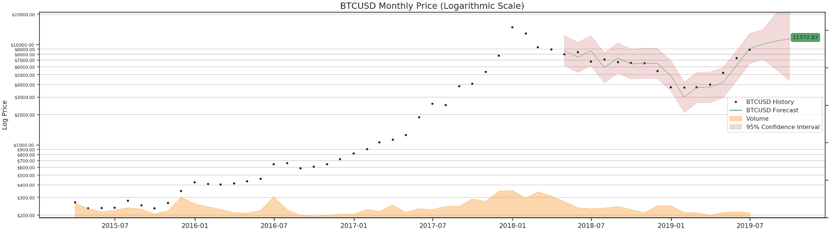
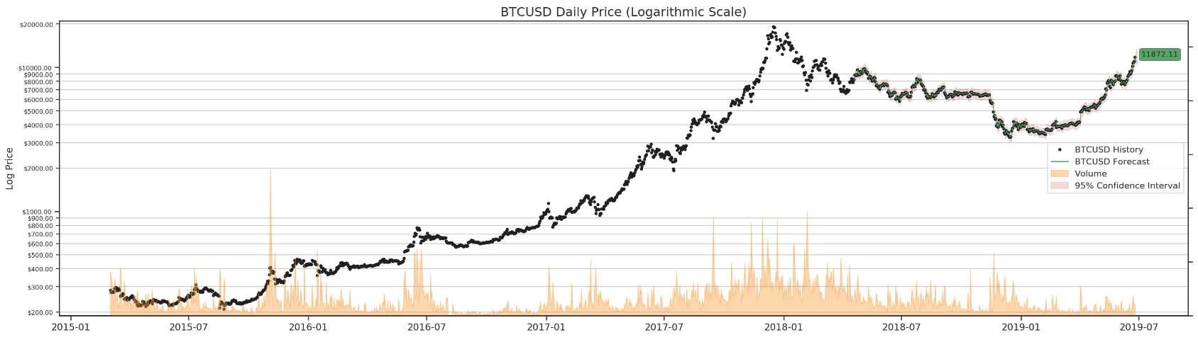
Finally, we can run it through all four data sets and forecast BTC in 3 days.
for df in df_list:
    render_results(df)
As mentioned earlier, we can try a different params combination for daily data.
render_results(d_df, params=(6, 1, 0))
I wish our results could be more accurate. Oh, well…
This might be the end of our series. We could explore a bit further by incoporating the seasonality into our model, and I will see if I can put up another post on that topic in the near future.
As always, all source code can be found on my github.
I hope you have enjoyed this series, and please do not forget to check out our quant channel. Feel free to shoot me a message if you have any questions/comments/proposals. Ciao!